Dynamic World data download

The real world is as dynamic as the people and natural processes that shape it. Dynamic World is a near realtime 10m resolution global land use land cover dataset, produced using deep learning, freely available and openly licensed. It is the result of a partnership between Google and the World Resources Institute, to produce a dynamic dataset of the physical material on the surface of the Earth. Dynamic World is intended to be used as a data product for users to add custom rules with which to assign final class values, producing derivative land cover maps.

Key innovations of Dynamic World

Near realtime data. Over 5000 Dynamic World image are produced every day, whereas traditional approaches to building land cover data can take months or years to produce. As a result of leveraging a novel deep learning approach, based on Sentinel-2 Top of Atmosphere, Dynamic World offers global land cover updating every 2-5 days depending on location.
Per-pixel probabilities across 9 land cover classes. A major benefit of an AI-powered approach is the model looks at an incoming Sentinel-2 satellite image and, for every pixel in the image, estimates the degree of tree cover, how built up a particular area is, or snow coverage if there’s been a recent snowstorm, for example.
Ten meter resolution. As a result of the European Commission’s Copernicus Programme making European Space Agency Sentinel data freely and openly available, products like Dynamic World are able to offer 10m resolution land cover data. This is important because quantifying data in higher resolution produces more accurate results for what’s really on the surface of the Earth.

App: www.dynamicworld.app
Paper: Dynamic World, Near real-time global 10m land use land cover mapping
Model: github
Geedata: Dynamic World V1

This tutorial explains how to download training data for Dynamic Earth using geemap

1. Import the necessary lib

import geemap
import ee
# ee.Authenticate()
geemap.set_proxy(port=33210)
ee.Initialize()
import os
import pandas   as  pd
import numpy as np
from  pyproj  import  CRS,Transformer

Map visualization

Map = geemap.Map()
Map.add_basemap('HYBRID')
region = ee.Geometry.BBox(-89.7088, 42.9006, -89.0647, 43.2167)
Map.centerObject(region)
image = geemap.dynamic_world_s2(region, '2021-01-01', '2022-01-01')
vis_params = {'bands': ['B4', 'B3', 'B2'], 'min': 0, 'max': 3000}
landcover = geemap.dynamic_world(region, '2021-01-01', '2022-01-01', return_type='hillshade')
Map.addLayer(landcover, {}, 'Land Cover')
Map.add_legend(title="Dynamic World Land Cover", builtin_legend='Dynamic_World')
Map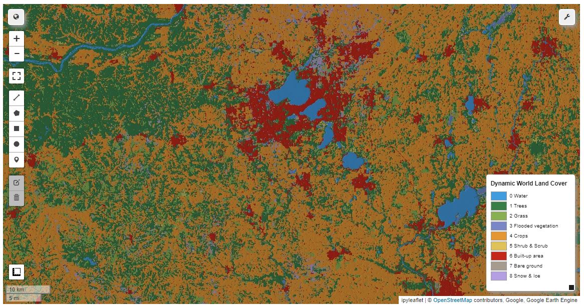

2. Download data

Construct a data combination with 8 bands, and use the data region, ID and other information provided by the paper to download image patches.

## cloud remove
def rmCloudByQA(image):
    qa = image.select('QA60')
    cloudBitMask = 1 << 10
    cirrusBitMask = 1 << 11 
    mask =qa.bitwiseAnd(cloudBitMask).eq(0)and(qa.bitwiseAnd(cirrusBitMask).eq(0))
    return image.updateMask(mask).toFloat().divide(1e4)
## convert utm to geo
def utm_to_geo(region,crs):
    strline=region.split('(',2)[-1].split(')',2)[0].split(', ')
    ymin,xmin=np.array(strline[0].split(' '))
    ymax,xmax=np.array(strline[2].split(' '))
    ocrs = CRS.from_string(crs)
    transformer = Transformer.from_crs(ocrs,'epsg:4326')
    ymin,xmin=transformer.transform(ymin,xmin)
    ymax,xmax=transformer.transform(ymax,xmax)
    return xmin,ymin,xmax,ymax
## Construct the 8-band data combination: Red,Green,Blue,Nir,Swir1,Swir2,MNDWI,Slope
def collection_cal(region,tiles,crs):
    s2Img = ee.ImageCollection('COPERNICUS/S2_SR')
    DEM = ee.Image('USGS/SRTMGL1_003')
    DEM_clip = DEM.setDefaultProjection(crs,None,10).clip(region)
    slope = ee.Terrain.slope(DEM_clip)
    S = s2Img.filter(ee.Filter.inList('system:index',tiles)).filterBounds(region).filter(ee.Filter.lt('CLOUDY_PIXEL_PERCENTAGE', 60)).map(rmCloudByQA).select('B.*').first().setDefaultProjection(crs,None,10)
    S2=S.clip(region)
    MNDWI = S2.normalizedDifference(['B3','B11']).rename(['MNDWI']).add(ee.Number(1))
    DBANDS=S2.select(['B4','B3','B2','B8','B11','B12'])
    final=DBANDS.addBands(MNDWI).addBands(slope).setDefaultProjection(crs,None,10)
    return final
## download function
def download_img(image,basename,out_dir):
    dw_id=basename+'.tif'
    # out_dir = os.path.expanduser(outdir)
    out_dem_stats = os.path.join(out_dir, dw_id)
    geemap.download_ee_image(image,out_dem_stats, num_threads=10,scale=10)

## visual check if if required
# Map = geemap.Map()
# Map.centerObject(region)
# Map.addLayer(region,{},'img')
# Map

The expert data in the table is downloaded here, and the label file can be downloaded through the link provided in the paper. During the download process, the file download may fail due to network reasons. In this case, you can try a few more times.

data=pd.read_csv('./expert.csv')
outdir='c:/temp/'
for index, row in data.iterrows():
    basename= row['dw_id']
    S2_GEE_ID= row['S2_GEE_ID']    
    crs= row['crs'] 
    tiles=[S2_GEE_ID]
    outfile = os.path.join(outdir, basename+'.tif')
    if os.path.exists(outfile):
    # if index < 3035:
        pass
    else:
        region= row['geometry']
        print(index,S2_GEE_ID)
        xmin,ymin,xmax,ymax=utm_to_geo(region,crs)
        regionClip = ee.Geometry.BBox(xmin,ymin,xmax,ymax)
        ImgTiles=collection_cal(regionClip,tiles,crs)
        download_img(ImgTiles,basename,outdir)
        # if index % 50==0:
        #     print('downloading......No.: '+str(index))

If you want to get the downloaded label data and related forms, you can follow the WeChat public account [45度科研人] and leave me a message！